Ako superpočítač pomáha odhaľovať tajomstvá buniek a zrýchľovať vývoj liekov
Predstavte si, že by ste mali ručne prezrieť milióny fotografií ľudských buniek a zistiť, ako presne reagujú na stovky rôznych chemických látok. Každá bunka sa správa trochu inak, mení svoj tvar v čase a reaguje na rôzne koncentrácie testovaných zlúčenín. Pre človeka, ale aj pre bežný počítač, je to úloha na celé dekády. V modernom medicínskom výskume však čas nemáme. Pacienti s vážnymi diagnózami potrebujú nové, bezpečnejšie a účinnejšie lieky hneď teraz.
Vďaka prelomovému výskumu publikovanému vo vedeckom časopise Machine Learning with Applications sa však podarilo niečo výnimočné. Slovenskí vedci z Fakulty prírodných vied a informatiky Univerzity Konštantína Filozofa v Nitre skrotili silu umelej inteligencie a superpočítačov, aby tento proces dramaticky zrýchlili.
Challenge
Pri hľadaní nových liekov vedci bežne využívajú takzvaný fenotypový skríning. Zjednodušene povedané: vezmú bunky, vystavia ich pôsobeniu testovanej látky a pod mikroskopom sledujú, čo sa stane.
Tradičný háčik bol v tom, že aby vedci v bunkách niečo jasne videli, museli ich najskôr chemicky „zafarbiť“ špeciálnymi fluorescenčnými látkami. Tento proces má však obrovské nevýhody:
- Je pomalý a drahý.
- Môže samotné bunky poškodiť alebo zmeniť ich správanie, čo skresľuje výsledky.
Vedci preto chceli prejsť na modernú digitálnu fázovo-kontrastnú mikroskopiu, ktorá bunky nepoškodzuje. Narazili však na obrovskú digitálnu stenu. Tieto snímky sú pre ľudské oko takmer nečitateľné a skrývajú obrovské množstvo dát. Navyše, určiť presný účinok látky, keď neviete, aká koncentrácia je tá správna a kedy presne sa prejaví, bolo s bežnou výpočtovou technikou prakticky nemožné.
Solution
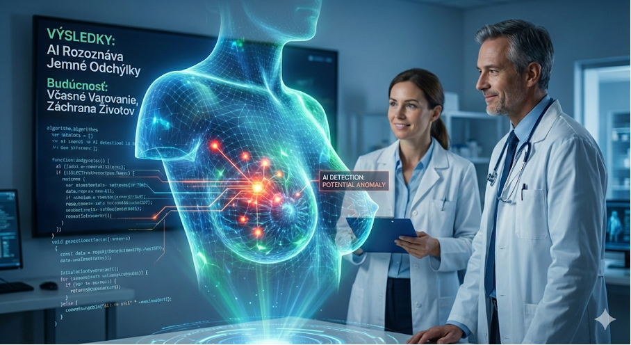
Tím výskumníkov prišiel s revolučným prístupom. Namiesto toho, aby umelá inteligencia (AI) analyzovala každý obrázok bunky samostatne, naučili ju premýšľať v súvislostiach. Navrhli metódu, ktorá dokáže spracovať celé skupiny snímok naraz – porovnáva rôzne koncentrácie látok a časové úseky, v ktorých na bunky pôsobili.
Aby sa však táto sofistikovaná neurónová sieť dokázala „naučiť“ rozpoznať správne vzorce a úspešne zatriediť viac ako 1 200 rôznych chemických zlúčenín, potrebovala gigantický výpočtový výkon. A práve tu zohral kľúčovú úlohu taliansky superpočítač Leonardo.
Vďaka prístupu k pokročilej superpočítačovej infraštruktúre (HPC) získal tím vedcov výkon tisícok bežných počítačov spojených do jedného celku. Tento superpočítačový motor umožnil v rekordne krátkom čase natrénovať AI model tak precízne, že dosiahol prelomovú presnosť pri analýze fázovo-kontrastných snímok bez potreby akéhokoľvek farbenia buniek.
Impact
Čo to znamená pre prax a pre nás všetkých?
- Koniec toxickým farbivám: Bunky môžeme sledovať v ich prirodzenom stave, vďaka čomu sú dáta o účinkoch budúcich liekov oveľa presnejšie.
- Radikálne zrýchlenie výskumu: Čas potrebný na analýzu miliónov mikroskopických obrazov sa skrátil z mesiacov na hodiny.
- Univerzálny nástroj (Transfer Learning): Vyvinutý model umelej inteligencie nie je jednoúčelový. Ukázalo sa, že ho možno okamžite „preklopiť“ a použiť na ďalšie kritické úlohy – napríklad na predpovedanie presného mechanizmu účinku neznámych liečiv alebo na okamžitú detekciu toho, či bunka na liečbu vôbec reaguje.
Celú štúdiu vrátane detailných dát nájdete priamo v knižnici Machine Learning with Applications.
Pohľad do budúcnosti
Tento úspech ukazuje, že éra, kedy sa lieky vyvíjali metódou pokus-omyl, sa definitívne končí. Spojenie biomedicínskeho výskumu, pokročilej umelej inteligencie a superpočítačov, ktoré zastrešuje NSCC Slovakia, otvára dvere k personalizovanej medicíne.
V budúcnosti by sa vďaka tejto technológii mohli testovať účinky liekov priamo na bunkách konkrétneho pacienta v reálnom čase, a nájsť tak najúčinnejšiu liečbu napríklad na onkologické či neurologické ochorenia bez zbytočných vedľajších účinkov. Slovensko vďaka HPC infraštruktúre a expertíze drží krok so svetovou špičkou a dokazuje, že superpočítače nie sú len pre teoretických fyzikov, ale zachraňujú ľudské životy.

 Keď sekundy v laboratóriu znamenajú roky života 11 Jul - Ako superpočítače pomáhajú odhaľovať tajomstvá buniek a zrýchľovať vývoj liekov